手把手教你，从零开始实现一个稀疏混合专家架构语言模型（MoE）

本文介绍了实现一个稀疏混合专家语言模型（MoE）的方法，详细解释了模型的实施过程，包括采用稀疏混合专家取代传统的前馈神经网络，实现 top-k 门控和带噪声的 top-k 门控，以及采用 Kaiming He 初始化技术。作者还说明了从 makemore 架构保持不变的元素，比如数据集处理、分词预处理和语言建模任务。最后还提供了一个 GitHub 仓库链接，用于实现模型的整个过程，是一本不可多得的实战教科书。

内容简介

在混合专家模型 Mixtral 发布后，混合专家模型（MoE）越来越受到人们的关注。在稀疏化的混合专家语言模型中，大部分组件都与传统的 transformers 相同。然而，尽管看似简单，但经验表明，稀疏混合专家语言模型训练的稳定性还存在着一些问题。

像这样易于修改的小规模实现可能有助于快速试验新方法。Hugging Face 上的一篇博客介绍了一种可配置的小规模稀疏 MoE 实施方法，也许有助于打算在这个方向深耕的研究者们进行快速试验自己的新方法，并且给出了基于 PyTorch 的详细代码：https://github.com/AviSoori1x/makeMoE/tree/main

机器之心对此进行了整理，以飨读者。

本文在 makemore 架构的基础上，进行了几处更改：

• 使用稀疏混合专家代替单独的前馈神经网络；

• Top-k 门控和有噪声的 Top-k 门控；

• 参数初始化使用了 Kaiming He 初始化方法，但本文的重点是可以对初始化方法进行自定义，这样就可以在 Xavier/Glorot 等初始化中进行选择。

同时，以下模块与 makemore 保持一致：

• 数据集、预处理（分词）部分以及 Andrej 最初选择的语言建模任务 - 生成莎士比亚文风的文本内容

• Casusal 自注意力机制

• 训练循环

• 推理逻辑

接下来逐步介绍实施方案，先从注意力机制开始。

因果缩放点积注意力机制

下面这段代码展示了自注意力机制的基本概念，并且侧重于使用经典的缩放点积自注意力（scaled dot product self-attention.）实现。在这一自注意力变体机制中，查询矩阵、键矩阵和值矩阵都来自相同的输入序列。同时为了确保自回归语言生成过程的完整性，特别是在纯解码器模型中，使用了一种掩码机制。

这种掩码机制非常关键，因为它可以掩盖当前 token 所处位置之后的任何信息，从而引导模型只关注序列的前面部分。这种了遮挡 token 后面内容的注意力被称为因果自注意力。值得注意的是，稀疏混合专家模型并不局限于仅有解码器的 Transformer 架构。事实上，这一领域的许多重要的成果都是围绕 T5 架构展开的，T5 架构也包含了 Transformer 模型中的编码器和解码器组件。

#This code is borrowed from Andrej Karpathy's makemore repository linked in the repo.The self attention layers in Sparse mixture of experts models are the same asin regular transformer models
torch.manual_seed(1337)B,T,C = 4,8,32 # batch, time, channelsx = torch.randn(B,T,C)
# let's see a single Head perform self-attentionhead_size = 16key = nn.Linear(C, head_size, bias=False)query = nn.Linear(C, head_size, bias=False)value = nn.Linear(C, head_size, bias=False)k = key(x)   # (B, T, 16)q = query(x) # (B, T, 16)wei =  q @ k.transpose(-2, -1) # (B, T, 16) @ (B, 16, T) ---> (B, T, T)
tril = torch.tril(torch.ones(T, T))#wei = torch.zeros((T,T))wei = wei.masked_fill(tril == 0, float('-inf'))wei = F.softmax(wei, dim=-1) #B,T,T
v = value(x) #B,T,Hout = wei @ v # (B,T,T) @ (B,T,H) -> (B,T,H)out.shape

torch.Size([4, 8, 16])

然后，因果自注意力和多头因果自注意力的代码可整理如下。多头自注意力并行应用多个注意力头，每个注意力头单独关注通道的一个部分（嵌入维度）。多头自注意力从本质上改善了学习过程，并由于其固有的并行能力提高了模型训练的效率。下面这段代码使用了 dropout 来进行正则化，来防止过拟合。

#Causal scaled dot product self-Attention Headn_embd = 64n_head = 4n_layer = 4head_size = 16dropout = 0.1
class Head(nn.Module):    """ one head of self-attention """
    def __init__(self, head_size):        super().__init__()        self.key = nn.Linear(n_embd, head_size, bias=False)        self.query = nn.Linear(n_embd, head_size, bias=False)        self.value = nn.Linear(n_embd, head_size, bias=False)        self.register_buffer('tril', torch.tril(torch.ones(block_size, block_size)))
        self.dropout = nn.Dropout(dropout)
    def forward(self, x):        B,T,C = x.shape        k = self.key(x)   # (B,T,C)        q = self.query(x) # (B,T,C)        # compute attention scores ("affinities")        wei = q @ k.transpose(-2,-1) * C**-0.5 # (B, T, C) @ (B, C, T) -> (B, T, T)        wei = wei.masked_fill(self.tril[:T, :T] == 0, float('-inf')) # (B, T, T)        wei = F.softmax(wei, dim=-1) # (B, T, T)        wei = self.dropout(wei)        # perform the weighted aggregation of the values        v = self.value(x) # (B,T,C)        out = wei @ v # (B, T, T) @ (B, T, C) -> (B, T, C)        return out

多头自注意力的实现方式如下：

#Multi-Headed Self Attentionclass MultiHeadAttention(nn.Module):    """ multiple heads of self-attention in parallel """
    def __init__(self, num_heads, head_size):        super().__init__()        self.heads = nn.ModuleList([Head(head_size) for _ in range(num_heads)])        self.proj = nn.Linear(n_embd, n_embd)        self.dropout = nn.Dropout(dropout)
    def forward(self, x):        out = torch.cat([h(x) for h in self.heads], dim=-1)        out = self.dropout(self.proj(out))        return out

创建一个专家模块

即一个简单的多层感知器

在稀疏混合专家架构中，每个 transformer 区块内的自注意力机制保持不变。不过，每个区块的结构发生了巨大的变化：标准的前馈神经网络被多个稀疏激活的前馈网络（即专家网络）所取代。所谓「稀疏激活」，是指序列中的每个 token 只被分配给有限数量的专家（通常是一个或两个）。

这有助于提高训练和推理速度，因为每次前向传递都会激活少数专家。不过，所有专家都必须存在 GPU 内存中，因此当参数总数达到数千亿甚至数万亿时，就会产生部署方面的问题。

#Expert moduleclass Expert(nn.Module):    """ An MLP is a simple linear layer followed by a non-linearity i.e. each Expert """
    def __init__(self, n_embd):        super().__init__()        self.net = nn.Sequential(            nn.Linear(n_embd, 4 * n_embd),            nn.ReLU(),            nn.Linear(4 * n_embd, n_embd),            nn.Dropout(dropout),        )
    def forward(self, x):        return self.net(x)

Top-k 门控的一个例子

门控网络，也称为路由，确定哪个专家网络接收来自多头注意力的 token 的输出。举个例子解释路由的机制，假设有 4 个专家，token 需要被路由到前 2 个专家中。首先需要通过线性层将 token 输入到门控网络中。该层将对应于（Batch size，Tokens，n_embed）的输入张量从（2，4，32）维度，投影到对应于（Batch size、Tokens，num_expert）的新形状：（2、4，4）。其中 n_embed 是输入的通道维度，num_experts 是专家网络的计数。

接下来，沿最后一个维度，找出最大的前两个值及其相应的索引。

#Understanding how gating worksnum_experts = 4top_k=2n_embed=32

#Example multi-head attention output for a simple illustrative example, consider n_embed=32, context_length=4 and batch_size=2mh_output = torch.randn(2, 4, n_embed)
topkgate_linear = nn.Linear(n_embed, num_experts) # nn.Linear(32, 4)
logits = topkgate_linear(mh_output)top_k_logits, top_k_indices = logits.topk(top_k, dim=-1)  # Get top-k expertstop_k_logits, top_k_indices

#output:(tensor([[[ 0.0246, -0.0190],          [ 0.1991,  0.1513],          [ 0.9749,  0.7185],          [ 0.4406, -0.8357]],          [[ 0.6206, -0.0503],          [ 0.8635,  0.3784],          [ 0.6828,  0.5972],          [ 0.4743,  0.3420]]], grad_fn=<TopkBackward0>), tensor([[[2, 3],          [2, 1],          [3, 1],          [2, 1]],          [[0, 2],          [0, 3],          [3, 2],          [3, 0]]]))

通过仅保留沿最后一个维度进行比较的前 k 大的值，来获得稀疏门控的输出。用负无穷值填充其余部分，在使用 softmax 激活函数。负无穷会被映射至零，而最大的前两个值会更加突出，且和为 1。要求和为 1 是为了对专家输出的内容进行加权。

zeros = torch.full_like(logits, float('-inf')) #full_like clones a tensor and fills it with a specified value (like infinity) for masking or calculations.sparse_logits = zeros.scatter(-1, top_k_indices, top_k_logits)sparse_logits

#outputtensor([[[   -inf,    -inf,  0.0246, -0.0190],         [   -inf,  0.1513,  0.1991,    -inf],         [   -inf,  0.7185,    -inf,  0.9749],         [   -inf, -0.8357,  0.4406,    -inf]],
        [[ 0.6206,    -inf, -0.0503,    -inf],         [ 0.8635,    -inf,    -inf,  0.3784],         [   -inf,    -inf,  0.5972,  0.6828],         [ 0.3420,    -inf,    -inf,  0.4743]]], grad_fn=<ScatterBackward0>)

gating_output= F.softmax(sparse_logits, dim=-1)gating_output

#ouputtensor([[[0.0000, 0.0000, 0.5109, 0.4891],         [0.0000, 0.4881, 0.5119, 0.0000],         [0.0000, 0.4362, 0.0000, 0.5638],         [0.0000, 0.2182, 0.7818, 0.0000]],
        [[0.6617, 0.0000, 0.3383, 0.0000],         [0.6190, 0.0000, 0.0000, 0.3810],         [0.0000, 0.0000, 0.4786, 0.5214],         [0.4670, 0.0000, 0.0000, 0.5330]]], grad_fn=<SoftmaxBackward0>)

使用有噪声的 top-k 门控以实现负载平衡

# First define the top k router module class TopkRouter(nn.Module):    def __init__(self, n_embed, num_experts, top_k):        super(TopkRouter, self).__init__()        self.top_k = top_k        self.linear =nn.Linear(n_embed, num_experts)        def forward(self, mh_ouput):        # mh_ouput is the output tensor from multihead self attention block        logits = self.linear(mh_output)        top_k_logits, indices = logits.topk(self.top_k, dim=-1)        zeros = torch.full_like(logits, float('-inf'))        sparse_logits = zeros.scatter(-1, indices, top_k_logits)        router_output = F.softmax(sparse_logits, dim=-1)        return router_output, indices

接下来使用下面这段代码来测试程序：

#Testing this out:num_experts = 4top_k = 2n_embd = 32
mh_output = torch.randn(2, 4, n_embd)  # Example inputtop_k_gate = TopkRouter(n_embd, num_experts, top_k)gating_output, indices = top_k_gate(mh_output)gating_output.shape, gating_output, indices#And it works!!

#output(torch.Size([2, 4, 4]), tensor([[[0.5284, 0.0000, 0.4716, 0.0000],          [0.0000, 0.4592, 0.0000, 0.5408],          [0.0000, 0.3529, 0.0000, 0.6471],          [0.3948, 0.0000, 0.0000, 0.6052]],          [[0.0000, 0.5950, 0.4050, 0.0000],          [0.4456, 0.0000, 0.5544, 0.0000],          [0.7208, 0.0000, 0.0000, 0.2792],          [0.0000, 0.0000, 0.5659, 0.4341]]], grad_fn=<SoftmaxBackward0>), tensor([[[0, 2],          [3, 1],          [3, 1],          [3, 0]],          [[1, 2],          [2, 0],          [0, 3],          [2, 3]]]))

尽管最近发布的 mixtral 的论文没有提到这一点，但本文的作者相信有噪声的 Top-k 门控机制是训练 MoE 模型的一个重要工具。从本质上讲，不会希望所有的 token 都发送给同一组「受欢迎」的专家网络。人们需要的是能在开发和探索之间取得良好平衡。为此，为了负载平衡，从门控的线性层向 logits 激活函数添加标准正态噪声是有帮助的，这使训练更有效率。

#Changing the above to accomodate noisy top-k gatingclass NoisyTopkRouter(nn.Module):    def __init__(self, n_embed, num_experts, top_k):        super(NoisyTopkRouter, self).__init__()        self.top_k = top_k        #layer for router logits        self.topkroute_linear = nn.Linear(n_embed, num_experts)        self.noise_linear =nn.Linear(n_embed, num_experts)
        def forward(self, mh_output):        # mh_ouput is the output tensor from multihead self attention block        logits = self.topkroute_linear(mh_output)
        #Noise logits        noise_logits = self.noise_linear(mh_output)
        #Adding scaled unit gaussian noise to the logits        noise = torch.randn_like(logits)*F.softplus(noise_logits)        noisy_logits = logits + noise
        top_k_logits, indices = noisy_logits.topk(self.top_k, dim=-1)        zeros = torch.full_like(noisy_logits, float('-inf'))        sparse_logits = zeros.scatter(-1, indices, top_k_logits)        router_output = F.softmax(sparse_logits, dim=-1)        return router_output, indices

再次尝试代码：

#Testing this out, again:num_experts = 8top_k = 2n_embd = 16
mh_output = torch.randn(2, 4, n_embd)  # Example inputnoisy_top_k_gate = NoisyTopkRouter(n_embd, num_experts, top_k)gating_output, indices = noisy_top_k_gate(mh_output)gating_output.shape, gating_output, indices#It works!!

#output(torch.Size([2, 4, 8]), tensor([[[0.4181, 0.0000, 0.5819, 0.0000, 0.0000, 0.0000, 0.0000, 0.0000],          [0.4693, 0.5307, 0.0000, 0.0000, 0.0000, 0.0000, 0.0000, 0.0000],          [0.0000, 0.4985, 0.5015, 0.0000, 0.0000, 0.0000, 0.0000, 0.0000],          [0.0000, 0.0000, 0.0000, 0.2641, 0.0000, 0.7359, 0.0000, 0.0000]],          [[0.0000, 0.0000, 0.0000, 0.6301, 0.0000, 0.3699, 0.0000, 0.0000],          [0.0000, 0.0000, 0.0000, 0.4766, 0.0000, 0.0000, 0.0000, 0.5234],          [0.0000, 0.0000, 0.0000, 0.6815, 0.0000, 0.0000, 0.3185, 0.0000],          [0.4482, 0.5518, 0.0000, 0.0000, 0.0000, 0.0000, 0.0000, 0.0000]]],        grad_fn=<SoftmaxBackward0>), tensor([[[2, 0],          [1, 0],          [2, 1],          [5, 3]],          [[3, 5],          [7, 3],          [3, 6],          [1, 0]]]))

创建稀疏化的混合专家模块

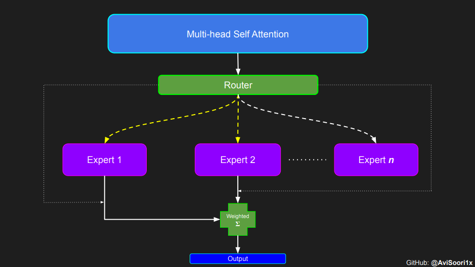
在获得门控网络的输出结果之后，对于给定的 token，将前 k 个值选择性地与来自相应的前 k 个专家的输出相乘。这种选择性乘法的结果是一个加权和，该加权和构成 SparseMoe 模块的输出。这个过程的关键和难点是避免不必要的乘法运算，只为前 k 名专家进行正向转播。为每个专家执行前向传播将破坏使用稀疏 MoE 的目的，因为这个过程将不再是稀疏的。

class SparseMoE(nn.Module):    def __init__(self, n_embed, num_experts, top_k):        super(SparseMoE, self).__init__()        self.router = NoisyTopkRouter(n_embed, num_experts, top_k)        self.experts = nn.ModuleList([Expert(n_embed) for _ in range(num_experts)])        self.top_k = top_k
    def forward(self, x):        gating_output, indices = self.router(x)        final_output = torch.zeros_like(x)
        # Reshape inputs for batch processing        flat_x = x.view(-1, x.size(-1))        flat_gating_output = gating_output.view(-1, gating_output.size(-1))
        # Process each expert in parallel        for i, expert in enumerate(self.experts):            # Create a mask for the inputs where the current expert is in top-k            expert_mask = (indices == i).any(dim=-1)            flat_mask = expert_mask.view(-1)
            if flat_mask.any():                expert_input = flat_x[flat_mask]                expert_output = expert(expert_input)
                # Extract and apply gating scores                gating_scores = flat_gating_output[flat_mask, i].unsqueeze(1)                weighted_output = expert_output * gating_scores
                # Update final output additively by indexing and adding                final_output[expert_mask] += weighted_output.squeeze(1)
        return final_output

运行以下代码来用样本测试上述实现，可以看到确实如此！

import torchimport torch.nn as nn
#Let's test this outnum_experts = 8top_k = 2n_embd = 16dropout=0.1
mh_output = torch.randn(4, 8, n_embd)  # Example multi-head attention outputsparse_moe = SparseMoE(n_embd, num_experts, top_k)final_output = sparse_moe(mh_output)print("Shape of the final output:", final_output.shape)

Shape of the final output: torch.Size([4, 8, 16])

需要强调的是，如上代码所示，从路由 / 门控网络输出的 top_k 本身也很重要。索引确定了被激活的专家是哪些， 对应的值又决定了权重大小。下图进一步解释了加权求和的概念。

模块整合

将多头自注意力和稀疏混合专家相结合，形成稀疏混合专家 transformer 块。就像在 vanilla transformer 块中一样，也要使用残差以确保训练稳定，并避免梯度消失等问题。此外，要采用层归一化来进一步稳定学习过程。

#Create a self attention + mixture of experts block, that may be repeated several number of times class Block(nn.Module):    """ Mixture of Experts Transformer block: communication followed by computation (multi-head self attention + SparseMoE) """
    def __init__(self, n_embed, n_head, num_experts, top_k):        # n_embed: embedding dimension, n_head: the number of heads we'd like        super().__init__()        head_size = n_embed // n_head        self.sa = MultiHeadAttention(n_head, head_size)        self.smoe = SparseMoE(n_embed, num_experts, top_k)        self.ln1 = nn.LayerNorm(n_embed)        self.ln2 = nn.LayerNorm(n_embed)
    def forward(self, x):        x = x + self.sa(self.ln1(x))        x = x + self.smoe(self.ln2(x))        return x

最后，将所有内容整合在一起，形成稀疏混合专家语言模型。

class SparseMoELanguageModel(nn.Module):
    def __init__(self):        super().__init__()        # each token directly reads off the logits for the next token from a lookup table        self.token_embedding_table = nn.Embedding(vocab_size, n_embed)        self.position_embedding_table = nn.Embedding(block_size, n_embed)        self.blocks = nn.Sequential(*[Block(n_embed, n_head=n_head, num_experts=num_experts,top_k=top_k) for _ in range(n_layer)])        self.ln_f = nn.LayerNorm(n_embed) # final layer norm        self.lm_head = nn.Linear(n_embed, vocab_size)
    def forward(self, idx, targets=None):        B, T = idx.shape
        # idx and targets are both (B,T) tensor of integers        tok_emb = self.token_embedding_table(idx) # (B,T,C)        pos_emb = self.position_embedding_table(torch.arange(T, device=device)) # (T,C)        x = tok_emb + pos_emb # (B,T,C)        x = self.blocks(x) # (B,T,C)        x = self.ln_f(x) # (B,T,C)        logits = self.lm_head(x) # (B,T,vocab_size)
        if targets is None:            loss = None        else:            B, T, C = logits.shape            logits = logits.view(B*T, C)            targets = targets.view(B*T)            loss = F.cross_entropy(logits, targets)
        return logits, loss
    def generate(self, idx, max_new_tokens):        # idx is (B, T) array of indices in the current context        for _ in range(max_new_tokens):            # crop idx to the last block_size tokens            idx_cond = idx[:, -block_size:]            # get the predictions            logits, loss = self(idx_cond)            # focus only on the last time step            logits = logits[:, -1, :] # becomes (B, C)            # apply softmax to get probabilities            probs = F.softmax(logits, dim=-1) # (B, C)            # sample from the distribution            idx_next = torch.multinomial(probs, num_samples=1) # (B, 1)            # append sampled index to the running sequence            idx = torch.cat((idx, idx_next), dim=1) # (B, T+1)        return idx

参数初始化对于深度神经网络的高效训练非常重要。由于专家中存在 ReLU 激活，因此这里使用了 Kaiming He 初始化。也可以尝试在 transformer 中更常用的 Glorot 初始化。杰里米 - 霍华德（Jeremy Howard）的《Fastai》第 2 部分有一个从头开始实现这些功能的精彩讲座：https://course.fast.ai/Lessons/lesson17.html

Glorot 参数初始化通常被用于 transformer 模型，因此这是一个可能提高模型性能的方法。

def kaiming_init_weights(m):    if isinstance (m, (nn.Linear)):         init.kaiming_normal_(m.weight)
model = SparseMoELanguageModel()model.apply(kaiming_init_weights)

本文作者使用 mlflow 跟踪并记录重要指标和训练超参数。

#Using MLFlowm = model.to(device)# print the number of parameters in the modelprint(sum(p.numel() for p in m.parameters())/1e6, 'M parameters')
# create a PyTorch optimizeroptimizer = torch.optim.AdamW(model.parameters(), lr=learning_rate)#mlflow.set_experiment("makeMoE")with mlflow.start_run():    #If you use mlflow.autolog() this will be automatically logged. I chose to explicitly log here for completeness    params = {"batch_size": batch_size , "block_size" : block_size, "max_iters": max_iters, "eval_interval": eval_interval,              "learning_rate": learning_rate, "device": device, "eval_iters": eval_iters, "dropout" : dropout, "num_experts": num_experts, "top_k": top_k }    mlflow.log_params(params)    for iter in range(max_iters):
        # every once in a while evaluate the loss on train and val sets        if iter % eval_interval == 0 or iter == max_iters - 1:            losses = estimate_loss()            print(f"step {iter}: train loss {losses['train']:.4f}, val loss {losses['val']:.4f}")            metrics = {"train_loss": losses['train'], "val_loss": losses['val']}            mlflow.log_metrics(metrics, step=iter)

        # sample a batch of data        xb, yb = get_batch('train')
        # evaluate the loss        logits, loss = model(xb, yb)        optimizer.zero_grad(set_to_none=True)        loss.backward()        optimizer.step()

8.996545 M parametersstep 0: train loss 5.3223, val loss 5.3166step 100: train loss 2.7351, val loss 2.7429step 200: train loss 2.5125, val loss 2.5233...
step 4999: train loss 1.5712, val loss 1.7508

记录训练和验证损失可以很好地指示训练的进展情况。该图显示，可能应该在 4500 次时停止（当验证损失稍微增加时）

接下来可以使用这个模型逐字符自回归地生成文本。

# generate from the model. Not great. Not too bad eithercontext = torch.zeros((1, 1), dtype=torch.long, device=device)print(decode(m.generate(context, max_new_tokens=2000)[0].tolist()))

DUKE VINCENVENTIO:If it ever fecond he town sue kigh now,That thou wold'st is steen 't.
SIMNA:Angent her; no, my a born Yorthort,Romeoos soun and lawf to your sawe with ch a woft ttastly defy,To declay the soul art; and meart smad.
CORPIOLLANUS:Which I cannot shall do from by born und ot cold warrike,What king we best anone wrave's going of heard and goodThus playvage; you have wold the grace....

本文参考内容：

在实施过程中，作者大量参考了以下出版物：

• 混合专家模型：https://arxiv.org/pdf/2401.04088.pdf

• 超大型神经网络：稀疏门控混合专家层：https://arxiv.org/pdf/1701.06538.pdf

• 来自 Andrej Karpathy 的原始 makemore 实现：https://github.com/karpathy/makemore

还可以尝试以下几种方法，来提高模型性能：

• 提高混合专家模块的效率；

• 尝试不同的神经网络初始化策略；

• 从字符级到子词级的分词；

• 对专家数量和 k 的取值（每个 token 激活的专家数量）进行贝叶斯超参数搜索。这可以归类为神经架构搜索。

• 优化专家能力。